You Can’t Spend Sharpe: Why Only Post-Tax Returns Matter
For Taxable LPs (High-Net-Worth Individuals, Family Offices, taxable corporations)

Returns after tax are what matters—Sharpe ratio is mostly for show. Legendary investors like Stanley Druckenmiller, George Soros, Warren Buffett, and Charlie Munger have all mocked the obsession with risk-adjusted metrics that allocators and LPs fixate on—because it’s disconnected from real, after-tax wealth. This mindset is starting to change, but not fast enough.
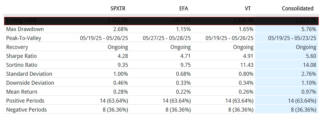
Just to be clear: if you’re a taxable investor, the Sharpe ratio is not a top metric to track. The biggest hedge funds raise from both tax-exempt giants (pensions, endowments, sovereigns) and taxable entities (family offices, individuals, corporates), but nearly every headline number, tear sheet, or “bragging rights” stat is pre-tax. As an investor who isn’t optimizing for Sharpe (though, for the record, AD Fund Management LP’s Sharpe for May was 5.60 versus SPXTR 4.28), I’ll talk my own book—Sharpe looks nice, but it’s irrelevant unless you’re tax-exempt. What actually matters is what lands in your account at year-end, not some risk-adjusted abstraction. What matters is the PnL, money in & money out POST TAX. Finally, I didn’t want to include gross returns from IBKR because the NAV and net returns are not finalized as for June 1st by Opus Fund Services.
If you’re paying taxes, you need to demand a different scoreboard. That especially goes for any fund that claims high Sharpe via rapid-fire, short-term trading. For a taxable LP, high turnover is a direct hit to compounding, and the difference between making money on paper and building real wealth. In this note, we’ll break down why after-tax returns—not Sharpe—are the only metric that matters for anyone who can’t duck the tax bill.
Let’s Define the Metrics First
Sharpe Ratio – Risk-Adjusted Return: The Sharpe ratio is a classic metric that evaluates how much excess return (above the risk-free rate) a portfolio delivers per unit of volatility (standard deviation of returns). Formulated by William F. Sharpe, it’s essentially a reward-to-risk measure: a higher Sharpe indicates more return for each unit of risk taken. For example, a fund with a Sharpe of 1 has historically delivered 1% of excess return for every 1% of return volatility. Institutional investors and allocators heavily rely on Sharpe ratios to compare managers on a level playing field – stripping out the effects of leverage or market beta and focusing on skill. It’s conventionally used in hedge fund due diligence and portfolio construction to ensure an investor is being compensated for the risk taken. A multi-strategy fund or quant fund boasting a Sharpe of 2+ is considered exceptional in risk-adjusted performance. Importantly, Sharpe is agnostic to who the investor is – it doesn’t change whether the LP is a pension (tax-exempt) or an individual; it’s purely a property of the investment track record.
Post-Tax Returns – Actual Investor Returns: Post-tax return is the net return after all taxes have been paid. In simplest terms, it’s the return that appears on an investor’s after-tax account balance, reflecting what they actually keep. This metric is especially relevant to high-net-worth and non-institutional LPs who must pay taxes on income, short-term capital gains, long-term gains, dividends, etc., often at different rates. Conventional use of post-tax performance metrics is common in the mutual fund world – for instance, the SEC requires U.S. mutual funds to publish standardized after-tax returns for 1-, 5-, and 10-year periods to help investors see the impact of taxes. Sophisticated taxable investors and their advisors will examine after-tax performance to decide whether a fund is worth it. For example, a quant equity fund might tout a 15% annual return pre-tax, but if an investor in the top tax bracket only nets ~9% after-tax due to high turnover distributions, that 9% is the more relevant figure for that investor’s true earnings. In short, post-tax return takes the “academic” performance and translates it into “real-life” outcomes.
Why Sharpe Ratios Can Misrepresent Wealth for Taxable Investors
A high Sharpe ratio signals an attractive pre-tax risk/reward profile – but for taxable investors, it can be a mirage in terms of actual wealth creation. The Sharpe ratio implicitly assumes no frictional costs like taxes. In reality, taxes can severely reduce the compounding of returns, meaning two strategies with identical Sharpe ratios could leave a taxable investor with very different ending wealth.
Mathematically, consider two portfolios each with an expected pre-tax return μ\mu and volatility σ\sigma, giving similar Sharpe ratios. If Portfolio A realizes gains frequently (short-term trading) and pays taxes each year at rate t, the investor’s after-tax growth rate each period is roughly μ after≈μ×(1−t) (assuming gains are taxed each period). Meanwhile, Portfolio B defers most gains and qualifies for lower long-term capital gains tax on realization, effectively getting taxed at a lower rate and less frequently. Sharpe ratio (pre-tax) would treat both as comparable (same μ,σ\mu, \sigma), but after-tax wealth accumulation will favor Portfolio B dramatically. The crux is that Sharpe focuses on the average excess return and volatility, not the compounding path of after-tax proceeds.
I believe after-tax returns, not gross returns, build wealth. In other words, it does not matter how much you make; it matters how much you keep. A taxable investor cares about the geometric growth of their capital after taxes. The Sharpe ratio, however, uses arithmetic mean returns in the numerator and doesn’t account for the tax drag that lowers that mean over time for the investor. Taxes are like a leak in the bucket – each time returns are realized, a portion is lost, and the base for compounding shrinks relative to a tax-free scenario. Sharpe won’t flag this leak because it looks only at pre-tax volatility-adjusted returns.
In fact, high turnover strategies can maintain a high Sharpe by delivering steady pre-tax gains, but they may be constantly bleeding out a portion of those gains to taxes. A taxable high-net-worth LP might find that a lower-Sharpe, low-turnover strategy yields more after-tax wealth than a higher-Sharpe trading strategy, once all taxes are accounted for. Empirical research backs this up: investors in top tax brackets will sometimes forego investments with higher before-tax returns in favor of ones with lower pre-tax returns if the latter deliver better after-tax outcomes. In other words, a rational taxable investor is interested in after-tax Sharpe, not just pre-tax Sharpe.
It’s also worth noting how different tax treatments for different return types can skew the picture. For example, in the U.S., long-term capital gains and qualified dividends are taxed at roughly 20%, whereas short-term gains and interest income can be taxed at ~37–40% for high earners. The Sharpe ratio doesn’t distinguish between a dollar of return coming from a long-term stock position vs. a dollar from short-term trading profits. But to the investor, the former dollar is worth a lot more after tax (80 cents kept vs. only ~60 cents on the short-term dollar). If a fund generates its returns in tax-advantaged ways, the investor’s after-tax risk-reward is better than Sharpe suggests. Conversely, if a fund’s returns come as ordinary income or short-term churn, the after-tax risk-reward is much worse than the Sharpe implies. This nuance was highlighted by researchers: due to favorable long-term capital gains rates and the ability to use loss harvesting, a taxable investor’s risk/reward slope is very different from a tax-exempt investor’s – the taxable investor effectively demands a higher pre-tax Sharpe to compensate for taxes. Sharpe ratio alone doesn’t capture that required adjustment.
Sharpe ratio is blind to taxes.
Case Study: Tax Impact on Two Similar-Sharpe Portfolios
Consider two long/short equity portfolios, both targeting a 10% annual pre-tax return with similar volatility (~10% standard deviation). On a pre-tax basis, each has a Sharpe around 1 (assuming a near-zero risk-free rate for simplicity). To an allocator looking at a performance summary, they might appear equally attractive. Now let’s examine the after-tax reality for a high-tax-bracket investor:
Portfolio A: High-Turnover Strategy – This portfolio actively trades and realizes its 10% return in full each year through short-term gains (taxed at 40%). At year-end, it distributes or realizes gains, and the investor pays 40% tax on that 10% profit. After-tax, the investor nets only 6% each year (keeping $0.60 of each $1 of gain). If you start with $100, after one year you have $106 after tax (instead of $110 pre-tax). After five years of compounding 6% after-tax annually, the $100 grows to about $133.8.
Portfolio B: Low-Turnover Tax-Efficient Strategy – This portfolio also achieves ~10% pretax annually on paper, but does so by holding positions longer and only realizing gains at the end of the 5-year period (assume gains qualify for long-term capital gains tax at 20%). So each year, it accrues 10% growth but does not trigger a taxable event until year 5. By the end of five years, the pre-tax portfolio value grows to about $161.1 (compounding 10% annually). Then the positions are liquidated, realizing the gain. The investor pays 20% tax on the $61.1 profit, losing about $12.2 to tax and ending with approximately $148.9 after tax.
Result: Both portfolios delivered a ~10% pretax return with similar volatility (so Sharpe ≈ 1). But Portfolio A’s investor ends with $133.8, whereas Portfolio B’s investor ends with $148.9 after five years – a difference of over 11% of the initial investment purely due to tax efficiency. In annualized terms, Portfolio A provided ~6% after-tax CAGR to the investor, while Portfolio B provided ~8.3% after-tax CAGR. This is a dramatic divergence in wealth creation, stemming not from skill or luck, but from tax drag.
Notably, Portfolio B’s after-tax Sharpe (if we computed it) would far exceed Portfolio A’s after-tax Sharpe, because the investor kept much more reward for the risk endured. Yet a standard performance report focusing on pre-tax Sharpe wouldn’t reveal this gap. This example mirrors real-world observations that taxes can sap 2% or more per year from equity returns for actively managed funds. Over longer horizons, that difference compounds significantly.
LP Segmentation: Institutional vs. Taxable Perspectives on Returns
Hedge funds often have a mix of institutional (tax-exempt) and individual or other taxable investors. These groups will interpret performance metrics differently:
Institutional LPs (Tax-Exempt Investors): Pension funds, endowments, foundations, and sovereign wealth funds generally pay no taxes on investment income or gains. A U.S. pension, for example, isn’t worried about capital gains taxes. This means an institutional LP evaluates a fund’s returns on a pre-tax basis – the Sharpe ratio, total pre-tax return, volatility, drawdowns, alpha relative to benchmarks, etc., are all directly relevant to their net outcome. They care about consistency, risk-adjusted returns, and hitting their required returns, and they do not need to discount those returns for tax leakage. For these investors, a dollar earned by the hedge fund is a dollar added to their assets (assuming the fund is structured properly to avoid unrelated business taxable income, etc., which is a separate structuring issue). As a result, fund managers often market to institutions highlighting high Sharpe ratios, alpha, and other pre-tax metrics – these directly align with the institutional investor’s experience. An institutional LP in London or New York or Singapore all share this: if they’re tax-exempt, a 10% return with Sharpe 1 is truly a 10% gain to them.
Taxable LPs (High-Net-Worth Individuals, Family Offices, taxable corporations): These investors must consider the tax implications of every return dollar. A 10% gain realized short-term might only net 6% after personal taxes, as we’ve discussed. Taxable LPs interpret a fund’s reported returns through the lens of “what will I actually keep?” They might mentally haircut a high-turnover fund’s returns knowing a large chunk will go to the tax man. For example, a U.S. individual in the top bracket will look at a strategy yielding lots of short-term gains and see an effective ~40% performance fee paid to the government on those gains. Taxable investors often zero in on after-tax return and tax efficiency: did the fund realize mostly long-term gains or harvest losses to offset gains? What is the “tax cost ratio” of the fund (the percentage of returns lost to tax) over time?
This segmentation often leads to differences in allocation decisions. An institutional LP might favor a high Sharpe, high-turnover quant strategy because it maximizes risk-adjusted returns pre-tax. A taxable LP might prefer a somewhat lower Sharpe strategy that’s more tax-friendly, or they might insist on investing through structures that mitigate taxes (for example, investing via an offshore feeder corporation or a life insurance wrapper to defer taxes). Indeed, many hedge funds set up separate vehicles for taxable investors – e.g., a “master-feeder” fund structure with an onshore feeder for U.S. taxable individuals (so they get a K-1 and pay taxes but can benefit from some loss pass-through) and an offshore feeder for non-U.S. and U.S. tax-exempt investors (to avoid certain taxes and UBTI issues). While both feeders see the same trading strategy, the taxable onshore feeder’s investors will be far more concerned with the nature of the income they get allocated.
Global differences also play a role. Taxable LPs in different jurisdictions face different rules: a tax-aware U.K. investor might be very sensitive to whether returns are income vs. capital gains (as their tax rates differ), whereas an investor in, say, a Gulf country with no personal capital gains tax wouldn’t care at all about that distinction. Some countries provide credits or exemptions via tax treaties (for instance, to avoid double taxation on foreign dividends); others do not. A fund that actively trades U.S. stocks might generate U.S. withholding tax on dividends for foreign investors or effectively connected income issues – these nuances will matter to those investors’ post-tax returns. Thus, the concept of “post-tax return” is inherently personal and jurisdiction-specific. Sophisticated LPs know their situation and will focus on metrics relevant to them. For example, an Australian family office (where franking credits on dividends matter) will interpret the fund’s returns differently than the Utah pension fund in the same strategy.
In conclusion, I want to end it with a quote from one of my idols Stanley Druckenmiller: “I’ve never used VAR. We had to use it at Soros to get banking lines from great companies like GS. But basically, [I’m] very unsophisticated - I watched my PnL every day and if it started acting in a strange manner in what I would expect out of a matrix, my antennae would go up. I’ve always used my PnL because I’ve found all those risks models are great until complete chaos happens and then all the correlations break down and they can suck you into a false sense of security. If you’re watching your PnL with your antennae up, and you’ve been doing it for 30 or 40 years - I’ve found it a much better warning system than some of these mathematical models which are useful, they’re just not useful when you need them.” Source
VAR (Value at Risk) is a statistical measure of the potential loss that an investment could experience within a specific timeframe and at a given confidence level. Sharpe Ratio is a measure of an investment's risk-adjusted return, indicating how much return an investor receives per unit of risk. In the end the only thing that matters is the PnL - money in, and money out. For taxable investors I’d recommend focusing on money in, and money out post-tax.